Neural Network somme theory
Author : maxime.savary@orange.com (v1.0 December 2020)
We introduce in this section the neural networks attached to the field of Deep Learning. The key point is the presentation of the backpropagation algorithm and the corresponding derivative calculations.
An effort has been made to obtain the clearest mathematical formulation, particularly in terms of indices. A more "packaged" mode from an algorithmic perspective is proposed in the two references below
Andrew NG courses https://www.youtube.com/playlist?list=PLLssT5z_DsK-h9vYZkQkYNWcItqhlRJLN (8.1 and following)
The complement can be found in the reference cited in the bibliography « Artificial Intelligence : A Modern Approach » and available here http://aima.cs.berkeley.edu/
Neuron Model
The objective is to build a classifying system from training data
An artificial neuron is a basic unit of a network which receives as input numbers $\{x_{1}, ..., x_{N}\}$ which are each multiplied by "weights" $\{w_1, ..., w_N\}$. If a neuron has $N$ Inputs, it has $N$ weights. These weighted data are added together to produce a logical unit. We add the bias which has the value $+1$ and its own weight $b$ then we calculate the output value $h_{\mathbf{w}}(x)$. This value is then compared to the expected value, here $y =\{0; 1\}$
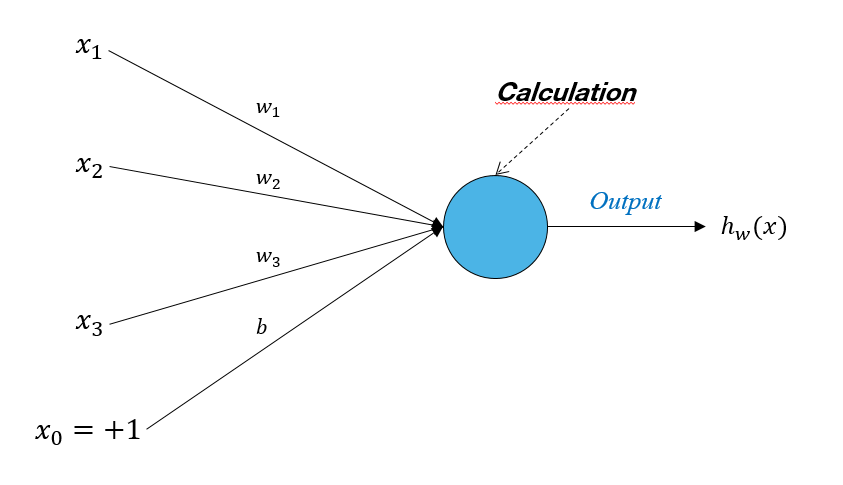
$h$ is broken down into :
- $z = b + \sum_{k=1}^{N}w_kx_{k}$
- $\sigma(z) = \frac{1}{1+e^{-z}}$
The bias $b$ :
- The bias acts on the neuron activation level. If we have $z = -20 + w_1x_1 + w_2x_2 + w_3x_3$ we have an inactive neuron as long as the weighted sum is not greater than $+20$
- To standardize the description, we will systematically put $x_0=+1$ for the input data linked to $b$ (his weight)
- We sometimes see the convention $b =w_0x_{0}$ to have a simpler writing of $z$ => $z = b + \sum_{k=1}^{N}w_kx_{k}$ or $z = \sum_{k=0}^{N}w_kx_{k}$
Activation function : $\sigma$ is called the activation function. Here we will use the sigmoid function which gives a nonlinear distribution between $0$ and $1$. But this function may be different depending on what we want to understand https://en.wikipedia.org/wiki/Activation_function
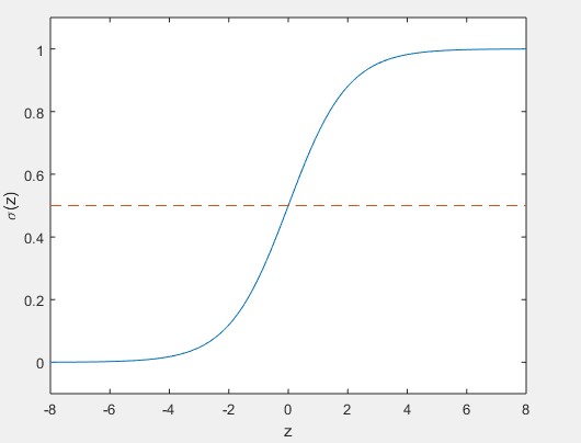
Function Derivate of $\sigma(z)$ :
$$\sigma '(z)=\frac{e^{-z}}{(1+e^{-z})^{2}} = \frac{1}{1+e^{-z}}(1-\frac{1}{1+e^{-z}})=\sigma(z)(1-\sigma(z)) \qquad \qquad (1.2)$$Neural Network
We build a multi-layer network by connecting "Layers" of neurons to each other. So the input of one neuron can be the output of another
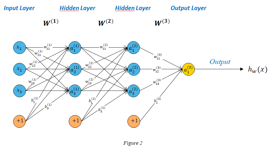
$4$ Layers:
- Input : First Layer. It takes the data and passes it to the next Layer without operation
- Hidden : They include the layers of neurons that are not seen in the "Training Set". They apply operations on the data received as inputs
- Output : It receives the data from the last Layer as input and produces the output data
We introduce here the following notations :
- $L$ Total number of Layers
- $s_{l}$ Number of Nodes (excepted bias) of Layer $l$
- $x \in \mathbb{R}^{N}$ input vector, $y\in \mathbb{R}^{K}$ output vector
- $W^{(l)}$ weight matrix connecting the Layers $l-1$ and $l$
- $w^{(l)}_{jk}$ weight connecting node $k$ of Layer $l-1$ and Node $j$ of Layer $l$ (The row index of the matrix therefore represents the index of the target node of the layer $l$)
- $b^{(l)}$ bias vector connecting Layers $l-1$ and $l$
- $z^{(l)}_{j} = b^{(l)}_{j} + \sum_{k=1}^{s_{l-1}}w^{(l)}_{jk}a^{(l-1)}_{k}$
- $a^{(l)}$ activation vector of Layer $l$
- $a^{(l)}_{j}$ the value calculated by the activation function of the unit $j$ in the Layer $l$ $$a^{(l)}_{j}=\sigma(b^{(l)}_{j} + \sum_{k=1}^{s_{l-1}}w^{(l)}_{jk}a^{(l-1)}_{k})$$
- $\sigma$ activation function. Here sigmoid function
For the network represented in figure 2 we have :
$$ \begin{aligned} &W^{(1 and 2)}\in \mathbb{R}^{3\times 3} \\ &W^{(3)}\in \mathbb{R}^{1\times 3} \\ &b^{(1 and 2)}\in \mathbb{R}^{1\times 3} \\ &b^{(3)}\in \mathbb{R}^{1\times 1} \\ \end{aligned} $$$$ \begin{aligned} &a^{(1)}_{1}=\sigma(b^{(1)}_{1} + w^{(1)}_{11}x_1 + w^{(1)}_{12}x_2 + w^{(1)}_{13}x_3) \\ &a^{(1)}_{2}=\sigma(b^{(1)}_{2} + w^{(1)}_{21}x_1 + w^{(1)}_{22}x_2 + w^{(1)}_{23}x_3) \\ &a^{(1)}_{3}=\sigma(b^{(1)}_{3} + w^{(1)}_{31}x_1 + w^{(1)}_{32}x_2 + w^{(1)}_{33}x_3)\\ \\ &a^{(2)}_{1}=\sigma(b^{(2)}_{1} + w^{(2)}_{11}a^{(1)}_{1} + w^{(2)}_{12}a^{(1)}_{2} + w^{(2)}_{13}a^{(1)}_{3}) \\ &a^{(2)}_{2}=\sigma(b^{(2)}_{2} + w^{(2)}_{21}a^{(1)}_{1} + w^{(2)}_{22}a^{(1)}_{2} + w^{(2)}_{23}a^{(1)}_{3}) \\ &a^{(2)}_{3}=\sigma(b^{(2)}_{3} + w^{(2)}_{31}a^{(1)}_{1} + w^{(2)}_{32}a^{(1)}_{2} + w^{(2)}_{33}a^{(1)}_{3}) \\ \end{aligned} $$$$h_{\mathbf{w}}(x)=a^{(3)}_{1}=\sigma(b^{(3)}_{1} + w^{(3)}_{11}a^{(2)}_{1} + w^{(3)}_{12}a^{(2)}_{2} + w^{(3)}_{13}a^{(2)}_{3})$$Using the previous standard notation, we will note : $$a^{(j)}_{i}=\sigma(z^{(j)}_{i})$$ $$z^{(j)}=\mathbf{w}^{(j-1)}.\mathbf{x}$$ $$a^{(j)}=\sigma(z^{(j)})$$
The Output Layer not necessary contains one unit. It can have several as below
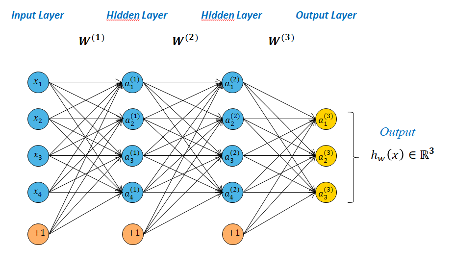
Here $h_{\mathbf{w}}(x) \in \mathbb{R}^{3}$
For example, we can build the network to have outputs of type
$h_{\mathbf{w}}(x)\approx\left(\begin{matrix} 1 \\ 0 \\ 0 \end{matrix} \right)$ => a Cat, $h_{\mathbf{w}}(x)\approx\left(\begin{matrix} 0 \\ 1 \\ 0 \end{matrix} \right)$ => a Dog, $h_{\mathbf{w}}(x)\approx\left(\begin{matrix} 0 \\ 0 \\ 1 \end{matrix} \right)$ => a Bird
Activation function
The activation function $\sigma$ is important because it allows to introduce nonlinearity into the neural network. It will make it possible to modelize a nonlinear problem.
Moreover it is important for the Gradient Descent and the calculations of derivatives of backpropagation algorithm - explained in the continuation - that this function is continuous and does not include jumps.
Example : The "XNOR"

We have here a network with 3 inputs and 2 Layers whose objective is to implement a [XNOR] (https://en.wikipedia.org/wiki/XNOR_gate) logic. The weights indicated in the diagram are fixed for illustration but a calculation by learning method is proposed below.
We have : $$ \begin{aligned} &x_1,x_2 \in \{0,1\} \\ \\ &a^{(1)}_{1}=\sigma(-30+20x_1+20x_2) \\ &a^{(1)}_{2}=\sigma(10-20x_1-20x_2) \\ &a^{(2)}_{1}=\sigma(-10+20a^{(1)}_{1}+20a^{(1)}_{2}) \\ \end{aligned} $$
| $x_1$ | $x_2$ | $a^{(1)}_{1}$ | $a^{(1)}_{2}$ | h(x) |
|---|---|---|---|---|
| 0 | 0 | 0 | 1 | $\approx$ 1 |
| 1 | 0 | 0 | 0 | $\approx$ 0 |
| 0 | 1 | 0 | 0 | $\approx$ 0 |
| 1 | 1 | 1 | 0 | $\approx$ 1 |
=> The Network with its weights and bias well simulate XNOR
Forward propagation
Function $h_{\mathbf{w},\mathbf{b}}(x)$ representing the Neural Network is a composed function which is expressed in matrix form :
$$ \begin{aligned} \mathbf{a}^{(0)}&= \mathbf{x}\\ \mathbf{z}^{(1)}&= \mathbf{W}^{(1)}.\mathbf{a}^{(0)}+\mathbf{b}^{(1)} \\ \mathbf{a}^{(1)} &= \sigma(\mathbf{z}^{(1)}) \\ \mathbf{z}^{(2)}&= \mathbf{W}^{(2)}.\mathbf{a}^{(1)}+\mathbf{b}^{(2)} \\ \mathbf{a}^{(2)} &= \sigma(\mathbf{z}^{(2)}) \\ &..... \\ \mathbf{a}^{(L)} &= h_{\mathbf{w},\mathbf{b}}(x) = \sigma(\mathbf{z}^{(L)})=Y \\ \end{aligned} $$The Cost Function
The objective of the training is to calculate the weights as well as possible to obtain a minimum error between the expected data and the data calculated by the neural network. For this we pass a training dataset $\{(x^{(1)},y^{(1)}),...,(x^{(m)},y^{(m)})\}$ in the neural network and we minimize a Cost function $E$ representing a measure of the total error between the calculated outputs and the expected ones
We have :
- $L$ Total nuber of Layers
- $x \in \mathbb{R}^{N}$ we have the norm $\left\|x\right\|_{2} = (\sum\limits_{i=1}^{N}{x^{2}_{i}} )^{\frac{1}{2} }$
- Training Set : $\{(x^{(1)},y^{(1)}),...,(x^{(m)},y^{(m)})\}$
- $E$ the Cost Function to minimize
- $h_{\mathbf{w},\mathbf{b}}(x)$ is the function representing the network and producing the output data
We define $E$ as the sum of the errors on all the training data by :
$$E(\mathbf{w},\mathbf{b}) = \frac{1}{m}\sum\limits_{t=1}^{m}E(\mathbf{w},\mathbf{b})_{t} \qquad \qquad (COST)$$with
$$E(\mathbf{w},\mathbf{b})_{t}=\frac{1}{2}\left\|y^{(t)}-h_{\mathbf{w},\mathbf{b}}(x^{(t)})\right\|^{2}_{2} \qquad \qquad (COSTt)$$Gradient Descent
Minimizing $E$ is therefore minimizing the error for each training data $(COSTt)$ then taking the average for all the data
We can see that $(COSTt)$ depends on weights $w^{(l)}_{jk}$, bias $b^{(l)}_{j}$ and values of activation functions $a^{(l)}_{j}$ calculated for each Node. But we can only "play" with the weights and the bias
This cost function can be used for both classification and regression problem. For Classification $y \in \{0,1\}$ the output is calculated by the Sigmoid function giving a distributuon in $[0,1]$. For a regression problem $y \in [0,1]$
The Cost Function $(COST)$ can be minimized (regarding $\mathbf{w}$ and $\mathbf{b}$) by the Gradient Descent Method Gradient Descent.
Minimizing is to "get down" in the opposite direction of the gradient which gives for each point the direction and the value of the greatest slope.
The figure below illustrates a Cost Function $E$ depending on 2 weights $w_{1}$ and $w_{2}$
- On the left the Cost function
- On the right a projection of the level lines and the gradient fields at each point. The gradient at a point is perpendicular to the level line
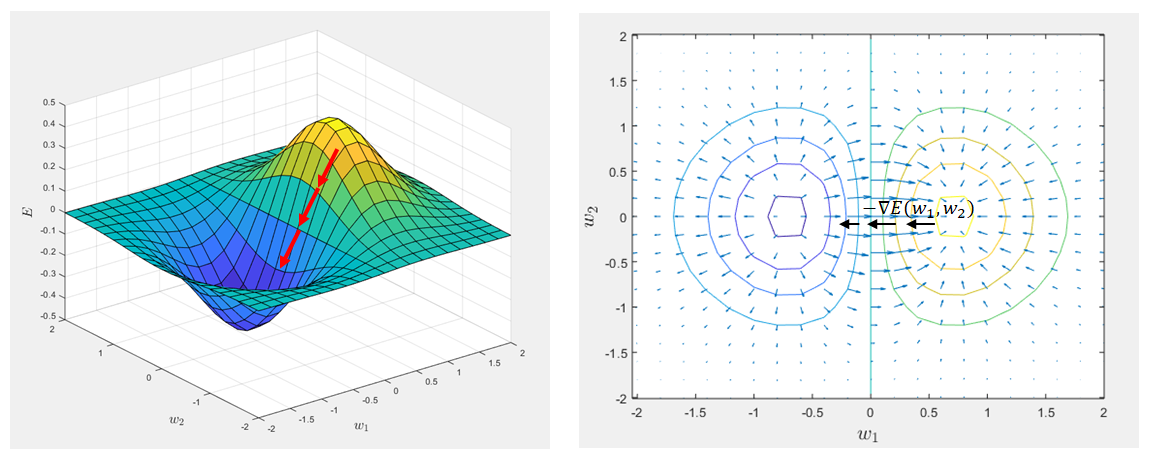
But unlike what is done here Gradient Descent there are Hidden Layers whose output and input values are not known. We only have the $\{(x^{(i)},y^{(i)})\}$ of the first and last Layer. We have to find the minimum of $(COST)$ regarding the weights $w^{(l)}_{jk}$ and $b^{(l)}_{j}$ going downhill "in the fog". We cannot modify the activation values, we can only play on the weights and bias !!!
We will therefore make a descent by calculating the gradients of $E(\mathbf{w},\mathbf{b})_{t}$ relativaly to $w$ and $b$ for each Layer $l$. Derivative calculations will allow us to see the influence that a disturbance of a given weight/bias has on the error, and therefore to be able to adjust. This is the backpropagation algoritm one of the creators is Yann Le Cun
$s_{l}$ being the Layer $l$ number of Nodes (without bias)
Stochastic Gradient Descent
An image character recognition neuron network can have millions of links. In that case calculating $(COSTt)$ on all training data and averaging can be very expensive. To avoid this we randomly take a subset of the training data set, then we calculate the gradients and so on. We decrease the descent step $\alpha$ as we approach the "valley bottom".
Thus appear the following notions :
- Batch : The Training Set
- Mini-Batch : Subset of Training Set
- Epochs : Number of Mini-Batch executed
In the following, we explain the Backpropagation algorithm by taking Mini-Batch = set of training data.
https://towardsdatascience.com/gradient-descent-algorithm-and-its-variants-10f652806a3
What about $E$ convexity ?
The gradient descent algorithm achieves the global minimum of the cost function $E$ only if it is convex. In the case of neural networks, this function is generally not convex and therefore comprises many "valleys" or minima. $E$ is convex if its Hessian matrix (second derivative) is positive-definite.
We will not do the calculation here but we can see it simply by noticing that the cost function is not modified if we exchange the weights $w^{l}_{jk}$ and $w^{l}_{jm}$ arriving at neuron $a^{l}_{j}$. We therefore have 2 different neural networks and we have found 2 local minima of $E$.

Despite this fact which can appear as problematic we will succeed by the method described below to build a correct network model. There is no formal explanation for this. Neural Networks work better than other methods but we do not know how to fully explain it. It is perhaps one of the doors allowing the production of a "magic" speech on AI
Backpropagation Algorithm
To do this we use an approach known as Backpropagation. It will consist in determining the influence of the different variables $z^{(l)}_{j}, a^{(l)}_{j}, b^{(l)}_{j}, w^{(l)}_{jk}$ on Cost Function $(COSTt)$ by calculating their derivatives.
Algorithm main steps :
- Randomly fix $w^{(l)}_{jk}$ and $b^{(l)}_{j}$ for $l \in {1,2,...,L}$
- Repeat until $epochs$ (nb iterations) or convergence condition on $E$
For each $ x=(x^{(t)},y^{(t)}) \in TrainingSet$
- Calculate $z^{(l),t}_{j}$ and $a^{(l),t}_{j}$ on all Layers $1,2,...,L$=> Forward propagation
- Calculate $E_{t}$ and first derivatives of the Output Layer $L$
$$\frac{\partial E_{t}}{\partial w^{(L)}_{jk}}$$ and $$\frac{\partial E_{t}}{\partial b^{(L)}_{j}}$$
backpropagate in order to calculate the derivatives for all the Layers $(L-1),(L-2), ... , 2$
$$\frac{\partial E_{t}}{\partial w^{(l)}_{jk}}$$ and $$\frac{\partial E_{t}}{\partial b^{(l)}_{j}}$$
Gradient Descent Update the weights and bias by averaging
The figure below represents the situation we have to understand at the level of derivatives calculation
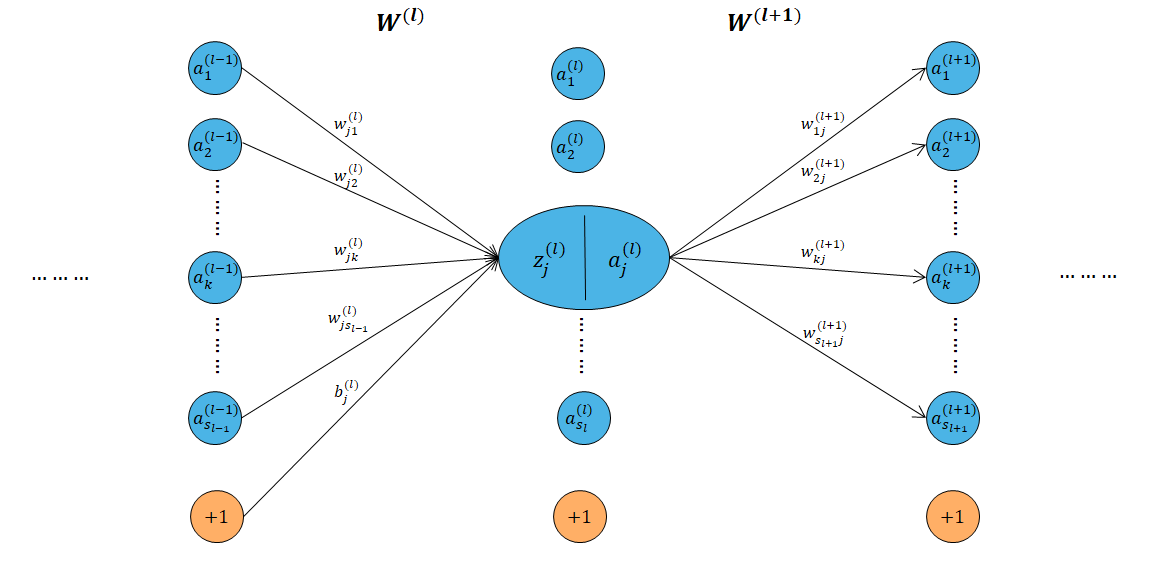
To simplify notations, we will omit the index $t$ referencing the training data $z^{(l),t}_{j}$ and $a^{(l),t}_{j}$ writing $z^{(l)}_{j}$ et $a^{(l)}_{j}$
Chain Rule
The Chain Rule on derivatives is the mathematical key point of backpropagation algorithm. It is used to calculate the influence of a variable on the output error.
It is based on derivatives of composite functions :
$$f(g(x))'=f'(g(x)).g'(x)$$putting $g(x)=y$ and $f(y)=z$ we have $$\frac{dz}{dx} = \frac{dz}{dy}.\frac{dy}{dx} $$
We will apply it to $(COSTt)$
Calculation of $\frac{\partial E_{t}}{\partial w^{(l)}_{jk}}$
We use here all the notations defined above + reminder :
$$z^{(l)}_{j} = b^{(l)}_{j} + \sum_{k}w^{(l)}_{jk}a^{(l-1)}_{k}$$$$a^{(l)}_{j} = \sigma(z^{(l)}_{j})$$Matrix form : $$\mathbf{z}^{(l)} = \mathbf{b}^{(l)} + \mathbf{w}^{(l)}\mathbf{a}^{(l-1)}$$ $$\mathbf{a}^{(l)} = \sigma(\mathbf{z}^{(l)})$$
The calculations are done with the training data fixed. So we have
$$E(\mathbf{w},\mathbf{b})_{t}=\frac{1}{2}\left\|y^{(t)}-a^{L})\right\|^{2}_{2}$$The derivative $\frac{\partial E_{t}}{\partial w^{(l)}_{jk}}$ evaluates the variation impact of $w^{(l)}_{jk}$ on final error $E_{t}$. The preceding figure shows that this variation impact $z^{(l)}_{j}$ which impacts $a^{(l)}_{j}$ which influence $E_{t}$. By applying the chain rule we see that the derivative therefore integrates 3 components.
Case $l=L$ Output Layer
$$z^{(L)}_{j} = b^{(L)}_{j} + \sum_{k}w^{(L)}_{jk}a^{(L-1)}_{k}$$We can write $(COSTt)$ as
$$E(\mathbf{w},\mathbf{b})_{t}=\frac{1}{2}\left\|y^{(t)}-a^{L})\right\|^{2}_{2}$$We simply get by derivation
$$ \begin{aligned} &\frac{\partial E_{t}}{\partial a^{(L)}_{j}}=(a^{(L)}_{j}-y^{(t)}) \\ &\frac{\partial z^{(L)}_{j}}{\partial w^{(L)}_{jk}}=a^{(L-1)}_{k} \\ &\frac{\partial a^{(L)}_{j}}{\partial z^{(L)}_{j}}=\sigma '(z^{(L)}_{j}) \\ \end{aligned} $$according to $(1.2)$
$$\sigma'(z)=\sigma(z)(1-\sigma(z))$$so $$\frac{\partial a^{(L)}_{j}}{\partial z^{(L)}_{j}}=a^{(L)}_{j}(1-a^{(L)}_{j})$$
$(3.1)$ is therefore written
$$\frac{\partial E_{t}}{\partial w^{(L)}_{jk}}=(a^{(L)}_{j}-y^{(t)})a^{(L)}_{j}(1-a^{(L)}_{j})a^{(L-1)}_{k} \qquad \qquad (3.2)$$General Case
We have as before
$$ \begin{aligned} &\frac{\partial a^{(l)}_{j}}{\partial z^{(l)}_{j}}=\sigma '(z^{(l)}_{j}) \\ &\frac{\partial z^{(l)}_{j}}{\partial w^{(l)}_{jk}}=a^{(l-1)}_{k} \\ \end{aligned} $$But here the derivative $\frac{\partial E_{t}}{\partial a^{(l)}_{j}}$ of $(3.1)$ is more complex. As we can see in the previous diagram we must evaluate how the variation of $a^{(l)}_{j}$ influence the following Nodes. Here the variation acts on all the nodes $a^{(l+1)}_{j}$ of the following Layer. By applying the chain rule we get
$$\frac{\partial E_{t}}{\partial a^{(l)}_{j}} = \sum\limits_{i=1}^{s_{l+1}}{\frac{\partial E_{t}}{\partial a^{(l+1)}_{i}}\frac{\partial a^{(l+1)}_{i}}{\partial z^{(l+1)}_{i}}\frac{\partial z^{(l+1)}_{i}}{\partial a^{(l)}_{j}} }$$$(3.1)$ is therefore written
$$\frac{\partial E_{t}}{\partial w^{(l)}_{jk}} = \frac{\partial E_{t}}{\partial a^{(l)}_{j}}\sigma '(z^{(l)}_{j})a^{(l-1)}_{k}$$$$\frac{\partial E_{t}}{\partial w^{(l)}_{jk}} = \sigma '(z^{(l)}_{j})a^{(l-1)}_{k}\sum\limits_{i=1}^{s_{l+1}}{\frac{\partial E_{t}}{\partial a^{(l+1)}_{i}}\frac{\partial a^{(l+1)}_{i}}{\partial z^{(l+1)}_{i}}\frac{\partial z^{(l+1)}_{i}}{\partial a^{(l)}_{j}} }$$with
$$\begin{aligned} &\frac{\partial a^{(l+1)}_{i}}{\partial z^{(l+1)}_{i}}=\sigma '(z^{(l+1)}_{i}) \\ &\frac{\partial z^{(l+1)}_{i}}{\partial a^{(l)}_{j}}=w^{(l+1)}_{ij} \\ \end{aligned}$$so
$$\frac{\partial E_{t}}{\partial w^{(l)}_{jk}} = \sigma '(z^{(l)}_{j})a^{(l-1)}_{k}\sum\limits_{i=1}^{s_{l+1}}{\frac{\partial E_{t}}{\partial a^{(l+1)}_{i}} \sigma '(z^{(l+1)}_{i})w^{(l+1)}_{ij}} \qquad \qquad (3.3)$$The calculated values :
- We know all terms $z^{(..)}_{j}, a^{(..)}_{j}$ calculated during propagation
- We know all weights $w^{(..)}_{ij}$
- And we know $\frac{\partial E_{t}}{\partial a^{(l+1)}_{i}}$ calculated previously => Here is the Key Point !!!
Calculation of $\frac{\partial E_{t}}{\partial b^{(l)}_{j}}$
We have $(3.1)$ equivalent by replacing the weight by the bias
$$\frac{\partial E_{t}}{\partial b^{(l)}_{j}} = \frac{\partial E_{t}}{\partial a^{(l)}_{j}}\frac{\partial a^{(l)}_{j}}{\partial b^{(l)}_{j}}=\frac{\partial E_{t}}{\partial a^{(l)}_{j}}\frac{\partial a^{(l)}_{j}}{\partial z^{(l)}_{j}}\frac{\partial z^{(l)}_{j}}{\partial b^{(l)}_{j}} \qquad \qquad (3.4)$$Case $l=L$ Output Layer
$$ \begin{aligned} &\frac{\partial E_{t}}{\partial a^{(L)}_{j}}=-(y^{(t)}-a^{(L)}_{j}) \\ &\frac{\partial a^{(L)}_{j}}{\partial z^{(L)}_{j}}=a^{(L)}_{j}(1-a^{(L)}_{j}) \\ &\frac{\partial z^{(L)}_{j}}{\partial b^{(L)}_{j}} = 1 \\ \end{aligned} $$$(3.1)$ is written :
$$\frac{\partial E_{t}}{\partial b^{(L)}_{j}} =-(y^{(t)}-a^{(L)}_{j})a^{(L)}_{j}(1-a^{(L)}_{j}) \qquad \qquad (3.5)$$General Case
$$ \begin{aligned} &\frac{\partial a^{(l)}_{j}}{\partial z^{(l)}_{j}}=\sigma '(z^{(l)}_{j}) \\ &\frac{\partial z^{(l)}_{j}}{\partial b^{(l)}_{j}}=1 \\ \end{aligned} $$$$\frac{\partial E_{t}}{\partial b^{(l)}_{j}} = \sigma '(z^{(l)}_{j})\sum\limits_{i=0}^{s_{l+1}}{\frac{\partial E_{t}}{\partial a^{(l+1)}_{i}}\frac{\partial a^{(l+1)}_{i}}{\partial z^{(l+1)}_{i}}\frac{\partial z^{(l+1)}_{i}}{\partial a^{(l)}_{j}} }$$thus
$$\frac{\partial E_{t}}{\partial b^{(l)}_{j}} = \sigma '(z^{(l)}_{j})\sum\limits_{i=0}^{s_{l+1}}{\frac{\partial E_{t}}{\partial a^{(l+1)}_{i}} \sigma '(z^{(l+1)}_{i})w^{(l+1)}_{ij}} \qquad \qquad (3.6)$$Example
Neural Network implementing XOR
The Objective is to implement an exclusive OR neural network whose truth table is :
| $A$ | $B$ | XOR |
|---|---|---|
| 0 | 0 | 0 |
| 1 | 0 | 1 |
| 0 | 1 | 1 |
| 1 | 1 | 0 |
It is a classification problem whose decision bound is not linear. We cannot separate the points by a straight line. The question we have to ask ourselves is how should I design the network to implement the function ?

If we take the simplest network called Sigmoid Perceptron

we have $$h_{\mathbf{w}}(x)=\sigma(w^{(1)}_{11}x_{1}+w^{(1)}_{12}x_{2}+b^{(1)}_{1})$$
In spite the nonlinearity of activation function (sigmoid) this network can simulate correctly a single decision boundary.
Knowing that we must have 2 separation boundaries, we build a Hidden Layer made up of 2 neurons which each will position a border. A detailed explanation and truth tables for each neuron can be found here http://toritris.weebly.com/perceptron-5-xor-how--why-neurons-work-together.html. The second layeur will do the "merge" and is made up of 1 neuron.
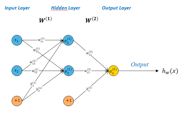
Note: We could create a different neural network, for example by introducing a second intermediate layer, and it would converge towards the same result. The backpropagation algorithm would balance the weights and bias minimizing the cost and the network output would "stick" to the inputs !!!
The python script below implements the backpropagation algorithm step by step. We deliberately made the calculations appear without using a compact instruction of the vector product type.
At the output we can see that the values predicted by the neural network correspond to the expected truth table and that the error $E$ has been minimized.
import numpy as np
import matplotlib.pyplot as plt


def sigmoid(x):
  return 1 / (1 + np.exp(-x))


def sigmoid_prime(x):
    return x * (1 - x)


# Intiatilization of weights and Bias for the XOR function (1 Hidden layer)
W1 = np.random.uniform(size=(2,2))
W2 = np.random.uniform(size=(1,2))
B1 = np.random.uniform(size=(2)).T
B2 = 0.1

# Batch : Training examples
X = np.array([[0,0],[0,1],[1,0],[1,1]])
y = np.array([0,1,1,0]).T

#Activation neurones
Z1 = np.zeros(2)
Z2 = np.zeros(1)
A1 = np.zeros(2)
A2 = np.zeros(1)

alpha = 0.15
m = 4 #number of trainning
epochs = 30000

costs = np.zeros(epochs)

output_calculated = np.zeros(4)

for j in range(epochs):
    cost_j = 0
    sum_dW1 = np.zeros((2,2))
    sum_dW2 = np.zeros((1,2))
    sum_dB1 = np.zeros((2,1))
    sum_dB2 = 0
    for i in range(X.shape[0]):
        #Forward Propagation
        Z1[0] = np.dot(W1[0,:],X[i]) + B1[0]
        Z1[1] = np.dot(W1[1,:],X[i]) + B1[1]
        A1[0] = sigmoid(Z1[0])
        A1[1] = sigmoid(Z1[1])
        Z2[0] = np.dot(W2[0,:],A1) + B2
        A2[0] = sigmoid(Z2[0])

        output_calculated[i] = A2[0]

        # Error
        cost_j = cost_j + 1/2*(A2[0] - y[i])**2
        #--------------Back Propagation--------------
        dW1 = np.zeros((2,2))
        dW2 = np.zeros((1,2))
        dB1 = np.zeros((2,1))
        dB2 = 0
        #Output Layer
        grad_pred = (A2[0] - y[i])
        dW2[0][0] =  grad_pred*A2[0]*(1 - A2[0])*A1[0]
        dW2[0][1] =  grad_pred*A2[0]*(1 - A2[0])*A1[1]
        dB2 = grad_pred*A2[0]*(1 - A2[0])

        #Hidden Layer
        dW1[0][0] = grad_pred*sigmoid_prime(A1[0])*X[i][0]*sigmoid_prime(A2[0])*W2[0][0]
        dW1[0][1] = grad_pred*sigmoid_prime(A1[0])*X[i][1]*sigmoid_prime(A2[0])*W2[0][0]
        dW1[1][0] = grad_pred*sigmoid_prime(A1[1])*X[i][0]*sigmoid_prime(A2[0])*W2[0][1]
        dW1[1][1] = grad_pred*sigmoid_prime(A1[1])*X[i][1]*sigmoid_prime(A2[0])*W2[0][1]
        dB1[0] = grad_pred*sigmoid_prime(A1[0])*sigmoid_prime(A2[0])*W2[0][0]
        dB1[1] = grad_pred*sigmoid_prime(A1[1])*sigmoid_prime(A2[0])*W2[0][1]

        #Sum Weights and Bias derivative for AVG
        sum_dW2[0][0] = sum_dW2[0][0] + dW2[0][0]
        sum_dW2[0][1] = sum_dW2[0][1] + dW2[0][1]
        sum_dB2 = sum_dB2 + dB2
        sum_dW1[0][0] = sum_dW1[0][0] + dW1[0][0]
        sum_dW1[0][1] = sum_dW1[0][1] + dW1[0][1]
        sum_dW1[1][0] = sum_dW1[1][0] + dW1[1][0]
        sum_dW1[1][1] = sum_dW1[1][1] + dW1[1][1]
        sum_dB1[0] = sum_dB1[0] + dB1[0]
        sum_dB1[1] = sum_dB1[1] + dB1[1]

    costs[j] = cost_j

    if cost_j < 0.005:
        break
    #update weights and bias
    W1[0][0] = W1[0][0] - (alpha/m)*sum_dW1[0][0]
    W1[0][1] = W1[0][1] - (alpha/m)*sum_dW1[0][1]
    W1[1][0] = W1[1][0] - (alpha/m)*sum_dW1[1][0]
    W1[1][1] = W1[1][1] - (alpha/m)*sum_dW1[1][1]
    W2[0][0] = W2[0][0] - (alpha/m)*sum_dW2[0][0]
    W2[0][1] = W2[0][1] - (alpha/m)*sum_dW2[0][1]
    B1[0] = B1[0] - (alpha/m)*sum_dB1[0]
    B1[1] = B1[1] - (alpha/m)*sum_dB1[1]
    B2 = B2 - (alpha/m)*sum_dB2


print('Final Hidden weights W1=',W1)
print('Final Hidden bias B1=',B1)
print('Final Hidden weights W2=',W2)
print('Final Hidden bias B2=',B2)
print("\nOutput calculated after ",epochs," epochs: ",output_calculated)

plt.xlabel('epochs')
plt.ylabel('Error')
plt.plot(np.arange(0,epochs), costs)
plt.show()
