Supervised Machine Learning
Author : maxime.savary@orange.com (v1.0 December 2020)
This part is a bit technical (Maths) but the objective here is to show how the problem is formalized and which entities must be calculated in the Algorithm
Notation : In formulas Vectors and Matrix are in Bold
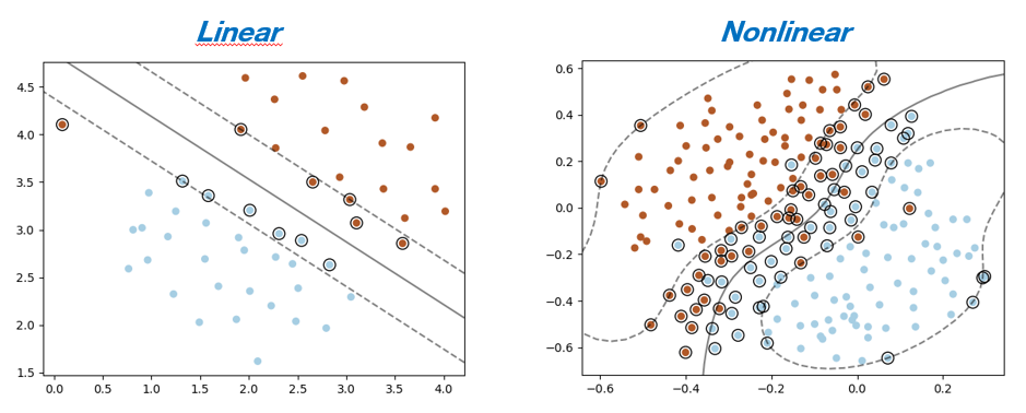
Classification with SVM
SVM (Support Vector Machine) is the most popular algorithm for classification methods grouped into "Kernels methods". It allows to position a "decision boundary"
The Support Vectors are elements of the "training set" which influence the "decision boundary" => These are the critical elements
The Problem => We have a Set of points $(\mathbf{x_0}, y_0), ..., (\mathbf{x_N}, y_N)$ with $\mathbf{x_i} \in \mathbb{R}^{N}$ and $y_{i} \in \{-1,1\}$
Network Bot Detection : For a specific IP
- $X = (nb\;request\;per\;seconds, error\;rate)$
- $Y = 1$ => IP is a Bot and $Y = -1$ => IP is not a Bot
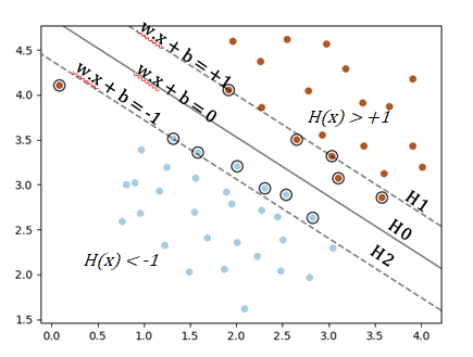
We are looking for an Hyperplane $h$ (a Line if $dim=2$) such as :
$$h: \mathbf{w}^T.\mathbf{x} + b = 0$$with $W$:weight vector and $b$: bias $\mathbf{w} = (w_{1}, ..., w_{N})^{T}$ et $\mathbf{x} = (x_{1}, ..., x_{N})^{T}$
$h(\mathbf{x}) = 0$ is the decision boundary
We add a « margin » constraint such as :
$$\begin{cases} h(\mathbf{x_i}) & \geq & 1 \;\; \text{for} \; y_i=+1\\ h(\mathbf{x_i}) & \leq & -1 \;\; \text{for} \; y_i=-1 \end{cases}$$These constraint state that each data point must lie on the correct side of the margin
The Classifier Function is given by $$G(x) = sign[\mathbf{w}^T.\mathbf{x} + b]$$
The algorithm objective is to find the separator plane ($\mathbf{w}$ and $\mathbf{b}$) and the margins that will maximize the bounds from training data. In other words, find the best border allowing to classify a data $x$ in the category $-1$ or $+1$
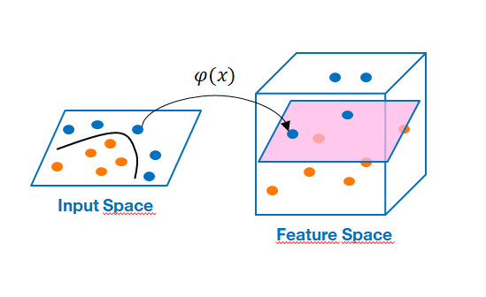
If the problem is nonlinear, we "dive" the data into a higher dimensional space (feature space $F$) by the "kernels" method and we look for a separating Hyperplane in this new space. This method is explained globally below + references: https://en.wikipedia.org/wiki/Kernel_method
SVM is computationally intensive and cannot be applied to a large amount of data
Linear Case
We have here a classification problem in which we suppose that the variable $\mathbf{x}$ follows a linear model
If $dim=N$, Euclidian distance is $$\lVert x \rVert=\sqrt{\sum_{i=1}^{N}x^{2}_{i}}$$
The distance beetween $H0$ and $H1$ :
$$\frac{\lvert \mathbf{w}^{T}.\mathbf{x}+b \rvert}{\lVert \mathbf{w} \rVert} = \frac{1}{\lVert \mathbf{w} \rVert}$$Equivalent formulation in dimension $n$ of the distance from a point to a line: $d = \frac{\lvert ax_{0}+by_{0}+c \lvert}{\sqrt{a^{2}+b^{2}}}$ https://en.wikipedia.org/wiki/Distance_from_a_point_to_a_plane
So, to maximize the margin $M = \frac{2}{\lVert \mathbf{w} \rVert}$ we have to minimize $\lVert \mathbf{w} \rVert$ with the condition that there must be no point between $H0$ and $H1$ either:
$$\begin{cases} \mathbf{w}^T.\mathbf{x_k} + b & \geq & 1 \;\; \text{if} \; y_k=+1\\ \mathbf{w}^T.\mathbf{x_k} + b & \leq & -1 \;\; \text{if} \; y_k=-1 \end{cases}$$which can be conbined : $y_k(\mathbf{w}^T.\mathbf{x_k} + b) \geq 1$ for $k=1,...,N$
Instead of maximizing $\frac{2}{\lVert w \rVert}$ we will minimizing $\frac{1}{2}\mathbf{w}^T.\mathbf{w} = \frac{1}{2}\lVert \mathbf{w}\rVert^{2}$
So we have to resolve :
Primary Form => $$\begin{cases} \min\frac{1}{2}\mathbf{w}^T.\mathbf{w}\\ y_i(\mathbf{w}^T.\mathbf{x_i} + b) & \geq & 1 & \text{for} & i=1, ..., N\end{cases}$$
From a mathematical point of view, this form is an optimization problem consisting in finding the extremums ($min$ / $max$) of a convex function under constraint
According to optimization theory (we do not develop the justification here. Presentation with example here https://www.svm-tutorial.com/2016/09/duality-lagrange-multipliers/) this problem can be solved by changing to its dual form and calculating the Lagrange multipliers. The solution of this dual problem is also the solution of the linear problem
For that we define the Lagrangian of the problem :
$$L(\mathbf{w},b,\boldsymbol{\alpha}) = \frac{1}{2}\mathbf{w}^T.\mathbf{w} - \sum_{k=1}^{N}\alpha_{k}(y_{k}(\mathbf{w}^{T}.\mathbf{x_{k}}+b) - 1)$$Therefore the problem is to minimize $L$ with respect to $w$, $b$ and to maximize it with respect to $\alpha$
Gradients of $L$ relatively to $w$, $b$ :
$$\begin{cases} \nabla_{w}L = \mathbf{w} - \sum_{k=1}^{N}\alpha_{k}y_{k}\mathbf{x_{k}} \\ \frac{\partial{L}}{\partial{b}} = -\sum_{k=1}^{N}\alpha_{k}y_{k} \end{cases}$$They must be zero. Which give :
$$\begin{cases} \sum_{k=1}^{N}\alpha_{k}y_{k}\mathbf{x_{k}} = \mathbf{w} \qquad \qquad &(1.1)\\ \sum_{k=1}^{N}\alpha_{k}y_{k} = 0 \qquad \qquad &(1.2)\end{cases}$$Important : The Lagrangian reformulation shows that $w$ is a linear combination of the examples
Developping $L$ and using $(1.1)$ and $(1.2)$ :
$$L(\mathbf{w},b,\boldsymbol{\alpha}) = \frac{1}{2}\mathbf{w}^T.\mathbf{w} - \sum_{k=1}^{N}\mathbf{w}^{T}.(\alpha_{k}y_{k}\mathbf{x_{k}}) - \sum_{k=1}^{N}\alpha_{k}y_{k}b + \sum_{k=1}^{N}\alpha_{k}$$$$L(\mathbf{w},b,\boldsymbol{\alpha}) = \sum_{k=1}^{N}\alpha_{k} - \frac{1}{2}\mathbf{w}^T.\mathbf{w} = \sum_{k=1}^{N}\alpha_{k} - \frac{1}{2}\sum_{i=1}^{N}\sum_{j=1}^{N}y_{i}y_{j}\alpha_{i}\alpha_{j}\mathbf{x_{i}}^{T}\mathbf{x_{j}}$$The formulated problem becomes :
$$\boxed{\\ \begin{cases} \underset{\alpha}{max}L(\boldsymbol{\alpha}) = \sum_{k=1}^{N}\alpha_{k} - \frac{1}{2}\sum_{i=1}^{N}\sum_{j=1}^{N}y_{i}y_{j}\alpha_{i}\alpha_{j}\mathbf{x_{i}}^{T}\mathbf{x_{j}}\\ \\ \text{with constraint} \quad \sum_{k=1}^{N}\alpha_{k}y_{k} = 0 \quad \text{and} \quad \alpha_{k} \geq 0\end{cases} \\ }$$Remarks :
- The algorithm to calculate the separation hyperplane consists in computing the $\alpha_{k}$ from the training data $(x_{k}, y_{k})$
- The $\alpha_{k}$ are calculated with libraries linked to convex quadratic optimization
Matrix form :
$\underset{\alpha}{max}L(\boldsymbol{\alpha}) = \mathbf{1}^{T}\boldsymbol{\alpha} - \frac{1}{2}\boldsymbol{\alpha}^{T}Q\boldsymbol{\alpha}$ with constraint $\mathbf{y}^{T}\boldsymbol{\alpha} = 0$ and $\alpha_{k} \geq 0$
$$Q = \begin{pmatrix} y_{1}y_{1}x_{1}^{T}x_{1} & ... & y_{1}y_{N}x_{1}^{T}x_{N} \\ ... & & ... \\ y_{N}y_{1}x_{N}^{T}x_{1} & & y_{N}y_{N}x_{N}^{T}x_{N} \\ \end{pmatrix}$$The method is very sensitive to the number of traning points : 1000 x 1000 if $N = 1000$ hence the advantage of having the most relevant data set as possible !!!
Once the $\alpha_{k}$ calculated. We rebuilt our information :
$$w = \sum_{k=1}^{N}\alpha_{k}y_{k}\mathbf{x_{k}}$$For points on margins H1 and H2 we have :
$$y_{k}(\mathbf{w}^{T}.\mathbf{x_{k}}+b) = 1$$hence $b$
Hyperplane equation : $$\boxed{ h(\mathbf{x}) = \sum_{k=1}^{N}\alpha_{k}y_{k}(\mathbf{x}^{T}.\mathbf{x_{k}}) + b }$$
The "soft margin"
In particular cases, some datas in the input set are misclassified. We therefore introduce a deviation tolerance called "soft margin"
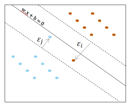
We allow an error based on separator hyperplane $\mathbf{w}^{T}\mathbf{x}+b$
$$\begin{cases} \mathbf{w}^T.\mathbf{x_k} + b \geq 1-\epsilon_{k} \;\; \text{if} \; y_k=+1\\ \mathbf{w}^T.\mathbf{x_k} + b \leq -1+\epsilon_{k} \;\; \text{if} \; y_k=-1\\ \epsilon_{k} \geq 0 \end{cases}$$$\epsilon_𝑖=0$ if no errors (the problem is linearly separable)
The problem becomes :
$$\begin{cases} \min\frac{1}{2}\mathbf{w}^T.\mathbf{w} + C\sum_{k=1}^{N}\epsilon_k\\ y_i(\mathbf{w}^T.\mathbf{x_i} + b) \geq 1 - \epsilon_k\quad \text{for} \, k=1, ..., N\\ \epsilon_k \geq 0 \end{cases}$$So we have a new parameter $C$ characterizing the margin tolerance => You can find it in Python algorithm signature (https://scikit-learn.org/stable/modules/generated/sklearn.svm.SVC.html)
Example :
- We load learning data set data.csv and data we want to classify data_test.csv
- We built the Model
- We classify the data_test
import pandas as pd
import matplotlib.pyplot as plt
import numpy as np
from sklearn import svm

df  = pd.read_csv("./datas/apibb-ML-introduction/data.csv")
df_test  = pd.read_csv("./datas/apibb-ML-introduction/data_test.csv")
x1 = df['X']
x2 =  df['Y']
y = df['Z']
x1_test = df_test['X']
x2_test =  df_test['Y']
y_test = df_test['Z']

X = np.column_stack((x1, x2))
X_test = np.column_stack((x1_test, x2_test))

model = svm.SVC(kernel='linear', C=1, gamma=1)
model.fit(X, y)
model.score(X, y)
#Predict Output
predicted= model.predict(X_test)
#print(predicted)

plt.scatter(X[:, 0], X[:, 1], c=y, s=30, cmap=plt.cm.Paired)


# plot the decision function
ax = plt.gca()
xlim = ax.get_xlim()
ylim = ax.get_ylim()

# create grid to evaluate model
xx = np.linspace(xlim[0], xlim[1], 30)
yy = np.linspace(ylim[0], ylim[1], 30)
YY, XX = np.meshgrid(yy, xx)
xy = np.vstack([XX.ravel(), YY.ravel()]).T
Z = model.decision_function(xy).reshape(XX.shape)

# plot decision boundary and margins
ax.contour(XX, YY, Z, colors='k', levels=[-1, 0, 1], alpha=0.5,
           linestyles=['--', '-', '--'])
# plot support vectors
ax.scatter(model.support_vectors_[:, 0], model.support_vectors_[:, 1], s=100,
           linewidth=1, facecolors='none', edgecolors='k')


plt.show()

Nonlinear case
Here we present the formulation of the mathematical problem without the "soft-margins". cf. $C$ parameter in algorithms
The kernels
In most of the problems encountered, the boundaries to be determined are not linear but they will be able to be calculated by introducing kernels method. It make possible to find nonlinear decision boundaries by immersing the data in a space of greater dimension in which the problem is linear !!! => This is called in ML the "kernel trick"
We will therefore be able to apply the previous method in an adequate space of higher dimension
"kernel trick" : Mathematics says that for any point in a space $\mathbb{R}^{n}$ a "kernel" function $k(x,y)$ (continuous, symmetric, positive-definite ) can be expressed as a dot product in a space $F=\mathbb{R}^{m}$
In the SVM problem, only the scalar product between the data has to be calculated. So if we can define how to calculate this product in the target space, we don't have to construct it explicitly. We use this to transform the computation of the scalar product (see example of kernels below)
A « kernel » is a function define by :
$$k : \mathbb{R}^{n}\times\mathbb{R}^{n} \rightarrow \mathbb{R}$$$$k(x,y) = <\varphi(x),\varphi(y)>$$with $$\varphi : \mathbb{R}^{n} \rightarrow \mathbb{R}^{m}$$
Thus we can calculate the dot product in the “Feature space $F$” without knowing the function $\varphi$ which is implicitly defined by $k$. In other words, we do not have to do the calculations (very expensive) in the very large space !!!
Concretely we construct a function $k$ which must correspond to a scalar product in a space of greater dimension
Kernels examples
In ML we generally use 3 kinds of Kernels :
- Linear : $k(x,y)=x^T.y$
- Polynomial : $k(x,y)=(x^T.y+1)^p$
- RBF (Radial Basis Function) : $k(x,y)=exp(-\frac{\lVert x-y \rVert^2}{\sigma^2})$
Dimension of $F$ space associated :
- Linear : if $n=10$ => $x$ has 10 parameters and $Dim(F) = 10$
- Polynomial : if $n=10$ and $p=5$ => $x$ has 10 parameters and $Dim(F) = \begin{pmatrix} 10+5 \\ 5\\ \end{pmatrix}= \frac{15!}{10!\,5!} = 3003$
- RBF : $Dim(F) = \infty$ !!!
Construction choosing a function $\varphi$ :
We choose $$\varphi(x) = \varphi(x_1,x_2) = (1, x^{2}_{1},x^{2}_{2},\sqrt{2}x_{1},\sqrt{2}x_{2},\sqrt{2}x_{1}x_{2})$$
$F$ dimension=6 and scalar product is :
$$<\varphi(x),\varphi(y)> = 1 + x^{2}_{1}y^{2}_{1} + x^{2}_{2}y^{2}_{2} + 2x_1y_1 + 2x_2y_2 + 2x_1x_2y_1y_2 = (1 + x_1y_1 + x_2y_2)^{2}$$$$<\varphi(x),\varphi(y)> = (1 + \mathbf{x}^{T}.\mathbf{y})^2` = k(x,y)$$Algebraically
Starting from the definition of the kernel functions and using the algebraic properties, we can build
$k(x,y)=exp(-\frac{\lVert x-y \rVert^2}{\sigma^2})$ which is continuous, symmetric, positive-definite
Developing by Taylor series we obtain :
$$\varphi(x) = e^{-\frac{x^{2}}{\sigma^{2}}}[1, \sqrt{\frac{1}{1!\sigma^{2}}}x, \sqrt{\frac{2}{2!\sigma^{4}}}x^{2}, ......]$$Here $k(x,y)$ calculates a scalar product in $dim=\infty$ without having to "visit" F !!!!
Problem reformulation
We reformulate the problem with the kernel method to adapt it to the nonlinear case
We are looking for : $$h(\mathbf{x}) = \mathbf{w}^T.\mathbf{\varphi(x)} + b$$ with $$y_{k}(\mathbf{w}^{T}.\mathbf{\varphi(x_{k})}+b) \geq 1$$
Either by using the same method as above, we end up with :
$$\boxed{\\ \begin{cases} \underset{\alpha}{max}L(\boldsymbol{\alpha}) = \sum_{k=1}^{N}\alpha_{k} - \frac{1}{2}\sum_{i=1}^{N}\sum_{j=1}^{N}y_{i}y_{j}\alpha_{i}\alpha_{j}\mathbf{\varphi(x_{i}})^{T}\varphi(\mathbf{x_{j}})\\ \text{with the constraint} \quad \sum_{k=1}^{N}\alpha_{k}y_{k} = 0 \quad \text{and} \quad \alpha_{k} \geq 0\end{cases} \\ }$$This is where the kernel function comes in, we replace with a kernel function that checks: $$k(\mathbf{x_i},\mathbf{y_i})=\mathbf{\varphi(x_i)}^T\varphi(\mathbf{y_i})$$
=> Hyperplane Equation : $$\boxed{\\ h(\mathbf{x}) = \sum_{k=1}^{N}\alpha_ky_kk(\mathbf{x_k},\mathbf{x})+b \\ }$$
Mathematical illustration of kernel method :
We have a Set of Points in $\mathbb{R}^{2}$ define by :
$$\begin{cases} y = 1 \quad \text{if} \; x^{2}+y^{2} < 1\\ y = -1 \quad \text{if} \; x^{2}+y^{2} > 1\end{cases}$$We dive the data into a higher space by giving:
$$\varphi: \mathbb{R}^{2} \rightarrow \mathbb{R}^{3}$$$$\varphi(x) = (x^{2}_{1}, x^{2}_{2}, \sqrt{2}x_{1}x_{2})$$We can easily calculate $k$ well corresponding to a scalar product in $\mathbb{R}^{3}$
$$k(x,y) = <\varphi(x), \varphi(y)> = (x^{2}_{1}y^{2}_{1}+ x^{2}_{2}y^{2}_{2} + 2x_1y_1x_2y_2)$$$$k(x,y) = <x,y>^2$$Matlab Program :
%Generate 100 points uniformly distributed in the unit disk.

rng(1); % For reproducibility
r = sqrt(rand(100,1)); % Radius
t = 2*pi*rand(100,1);  % Angle
data1 = [r.*cos(t), r.*sin(t)]; % Points


%Generate 100 points uniformly distributed in the annulus
r2 = sqrt(3*rand(200,1)+1); % Radius
t2 = 2*pi*rand(200,1);      % Angle
data2 = [r2.*cos(t2), r2.*sin(t2)]; % points

%Z
zdata1 = sqrt(2).*data1(:,1).*data1(:,2);
zdata2 = sqrt(2).*data2(:,1).*data2(:,2);

figure;
scatter(data1(:,1),data1(:,2),'r','filled')
hold on
scatter(data2(:,1),data2(:,2),'b','filled')
axis equal
hold off

figure;
scatter3(data1(:,1).^2,data1(:,2).^2,zdata1,'r','filled')
hold on
scatter3(data2(:,1).^2,data2(:,2).^2,zdata2,'b','filled')
xlabel('x1^2')
ylabel('x2^2')
zlabel('sqrt(2)x1x2')
hold off

%surface plot
hold on
[x, z] = meshgrid(0:0.1:4,-3:0.1:3);
Yv = @(x) 1-x;
mesh(x,Yv(x),z);
hold off
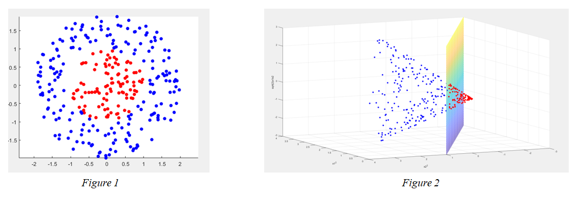
figure 1 represents points in input space. The separation boundary is nonlinear. figure 2 represents all the points in the feature space $F = \mathbb{R}^{3}$ provided with the coordinate system given by $\varphi(x) = (x^{2}_{1}, x^{2}_{2}, \sqrt{2}x_{1}x_{2})$ => The separation boundary is linear and given by the plane of equation $x^{2}+y^{2} = 1$
Python Demo of classification problem :
- Machine Learning Pyhton package is scikit-learn : https://scikit-learn.org/stable/index.html
- SVM methods : https://scikit-learn.org/stable/modules/svm.html
In Python 3 methods for SVM : kernel=Linear|Poly|RBF
We see here the interest of understanding what is played out mathematically : If you choose kernel
Polyin your Python program, you know that the degreepgives the dimension of the arrival space in which we find the separator plane $H$
In the case kernel=Linear, It is the standard scalar product => $F$ is identical to input space. We find C which is the margin tolerance
Linear : $k(x,y)=x^Ty$
model = svm.SVC(kernel='linear', C=10)
Polynomial : $k(x,y)=(x^Ty+1)^p$
model = svm.SVC(kernel='poly', degree=5, C=10)
RBF (Gaussian) : $k(x,y)=exp(-\frac{\lVert x-y \rVert^2}{\sigma^2})$ with $\gamma = \sigma^2$
model = svm.SVC(kernel='rbf', random_state=0, gamma=0.1, C=10)
The gamma parameter : « Each point influence » => If too high we will have boundaries close to each point
C parameter :
- small implies an important boundary => Low error tolerance
- big implies a weak boundary => High error tolerance
In following demo :
- 100 points are generated uniformly in the unit disc $x^2+y^2<1$ AND we tagged inside to +1
- we generate 200 points uniformly in $1<x^2+y^2<2$ AND we tagged inside to -1
Linear
import numpy as np
import matplotlib.pyplot as plt
from sklearn import svm


#Generate 100 points uniformly distributed in the unit disk.
r = np.sqrt(np.random.rand(100,1))
t = 2*np.pi*(np.random.rand(100,1))
data1_x1 = r*np.cos(t)
data1_x2 = r*np.sin(t)
data1_y = np.ones(100)

r2 = np.sqrt(3*np.random.rand(200,1) + 1)
t2 = 2*np.pi*(np.random.rand(200,1))
data2_x1 = r2*np.cos(t2)
data2_x2 = r2*np.sin(t2)
data2_y = -np.ones(200)

data1 = np.column_stack((data1_x1, data1_x2))
data2 = np.column_stack((data2_x1, data2_x2))
X = np.concatenate((data1, data2), axis=0)
y = np.concatenate((data1_y, data2_y), axis=0)


model = svm.SVC(kernel='linear', C=10)

model.fit(X, y)
model.score(X, y)

plt.scatter(data1_x1,data1_x2)
plt.scatter(data2_x1,data2_x2)

# plot the decision function
ax = plt.gca()
xlim = ax.get_xlim()
ylim = ax.get_ylim()


# create grid to evaluate model
xx = np.linspace(xlim[0], xlim[1], 30)
yy = np.linspace(ylim[0], ylim[1], 30)
YY, XX = np.meshgrid(yy, xx)
xy = np.vstack([XX.ravel(), YY.ravel()]).T
Z = model.decision_function(xy).reshape(XX.shape)


# plot decision boundary and margins
ax.contour(XX, YY, Z, colors='k', levels=[-1, 0, 1], alpha=0.5,
           linestyles=['--', '-', '--'])
# plot support vectors
ax.scatter(model.support_vectors_[:, 0], model.support_vectors_[:, 1], s=100,
           linewidth=1, facecolors='none', edgecolors='k')


plt.show()

Polynomial p=2
import numpy as np
import matplotlib.pyplot as plt
from sklearn import svm


#Generate 100 points uniformly distributed in the unit disk.
r = np.sqrt(np.random.rand(100,1))
t = 2*np.pi*(np.random.rand(100,1))
data1_x1 = r*np.cos(t)
data1_x2 = r*np.sin(t)
data1_y = np.ones(100)

r2 = np.sqrt(3*np.random.rand(200,1) + 1)
t2 = 2*np.pi*(np.random.rand(200,1))
data2_x1 = r2*np.cos(t2)
data2_x2 = r2*np.sin(t2)
data2_y = -np.ones(200)

data1 = np.column_stack((data1_x1, data1_x2))
data2 = np.column_stack((data2_x1, data2_x2))
X = np.concatenate((data1, data2), axis=0)
y = np.concatenate((data1_y, data2_y), axis=0)


model = svm.SVC(kernel='poly', degree=2, C=10, gamma='scale')


model.fit(X, y)
model.score(X, y)

plt.scatter(data1_x1,data1_x2)
plt.scatter(data2_x1,data2_x2)

# plot the decision function
ax = plt.gca()
xlim = ax.get_xlim()
ylim = ax.get_ylim()


# create grid to evaluate model
xx = np.linspace(xlim[0], xlim[1], 30)
yy = np.linspace(ylim[0], ylim[1], 30)
YY, XX = np.meshgrid(yy, xx)
xy = np.vstack([XX.ravel(), YY.ravel()]).T
Z = model.decision_function(xy).reshape(XX.shape)


# plot decision boundary and margins
ax.contour(XX, YY, Z, colors='k', levels=[-1, 0, 1], alpha=0.5,
           linestyles=['--', '-', '--'])
# plot support vectors
ax.scatter(model.support_vectors_[:, 0], model.support_vectors_[:, 1], s=100,
           linewidth=1, facecolors='none', edgecolors='k')


plt.show()

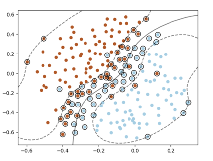
RBF
import numpy as np
import matplotlib.pyplot as plt
from sklearn import svm


#Generate 100 points uniformly distributed in the unit disk.
r = np.sqrt(np.random.rand(100,1))
t = 2*np.pi*(np.random.rand(100,1))
data1_x1 = r*np.cos(t)
data1_x2 = r*np.sin(t)
data1_y = np.ones(100)

r2 = np.sqrt(3*np.random.rand(200,1) + 1)
t2 = 2*np.pi*(np.random.rand(200,1))
data2_x1 = r2*np.cos(t2)
data2_x2 = r2*np.sin(t2)
data2_y = -np.ones(200)

data1 = np.column_stack((data1_x1, data1_x2))
data2 = np.column_stack((data2_x1, data2_x2))
X = np.concatenate((data1, data2), axis=0)
y = np.concatenate((data1_y, data2_y), axis=0)


model = svm.SVC(kernel='rbf', random_state=0, gamma=0.1, C=10)


model.fit(X, y)
model.score(X, y)

plt.scatter(data1_x1,data1_x2)
plt.scatter(data2_x1,data2_x2)

# plot the decision function
ax = plt.gca()
xlim = ax.get_xlim()
ylim = ax.get_ylim()


# create grid to evaluate model
xx = np.linspace(xlim[0], xlim[1], 30)
yy = np.linspace(ylim[0], ylim[1], 30)
YY, XX = np.meshgrid(yy, xx)
xy = np.vstack([XX.ravel(), YY.ravel()]).T
Z = model.decision_function(xy).reshape(XX.shape)


# plot decision boundary and margins
ax.contour(XX, YY, Z, colors='k', levels=[-1, 0, 1], alpha=0.5,
           linestyles=['--', '-', '--'])
# plot support vectors
ax.scatter(model.support_vectors_[:, 0], model.support_vectors_[:, 1], s=100,
           linewidth=1, facecolors='none', edgecolors='k')


plt.show()
